Experimental Physics

Beginner

Physics is not just about solving equations on a blackboard; it is an experimental science. To prove a theory, we must perform experiments and take measurements. However, no measurement in the real world is ever completely perfect.

Accuracy vs. Precision

When we take measurements, we must understand two important concepts:

Accuracy: How close your measurement is to the true, accepted value.
Precision: How close a series of measurements are to one another, regardless of whether they are correct.

Accuracy vs Precision on a Dartboard

Significant Figures

To show how reliable our measurements are, we use significant figures. These are the digits in a number that carry meaningful information about its precision.

For example, if you measure a book's length with a standard ruler, you might write $24.3\text{ cm}$ . The $2$ and $4$ are certain, while the $.3$ is an estimate. Writing $24.300\text{ cm}$ would imply your ruler is far more precise than it actually is.

Basic Rules for Counting Significant Figures:

All non-zero digits are significant (e.g., $438$ has three).
Zeros between non-zero digits are significant (e.g., $105$ has three).
Leading zeros are not significant (e.g., $0.0025$ has only two).
Trailing zeros to the right of a decimal point are significant (e.g., $4.70$ has three).

To understand how these values are cataloged under standard systems of measurement, see the guide on Units and Dimensions.

Intermediate

When standard rulers are too coarse to measure tiny objects, we use specialized laboratory instruments like the Vernier Caliper.

Vernier Calipers

A Vernier caliper consists of a main scale and a sliding auxiliary scale (the Vernier scale) that allows us to read fractions of the smallest division on the main scale.

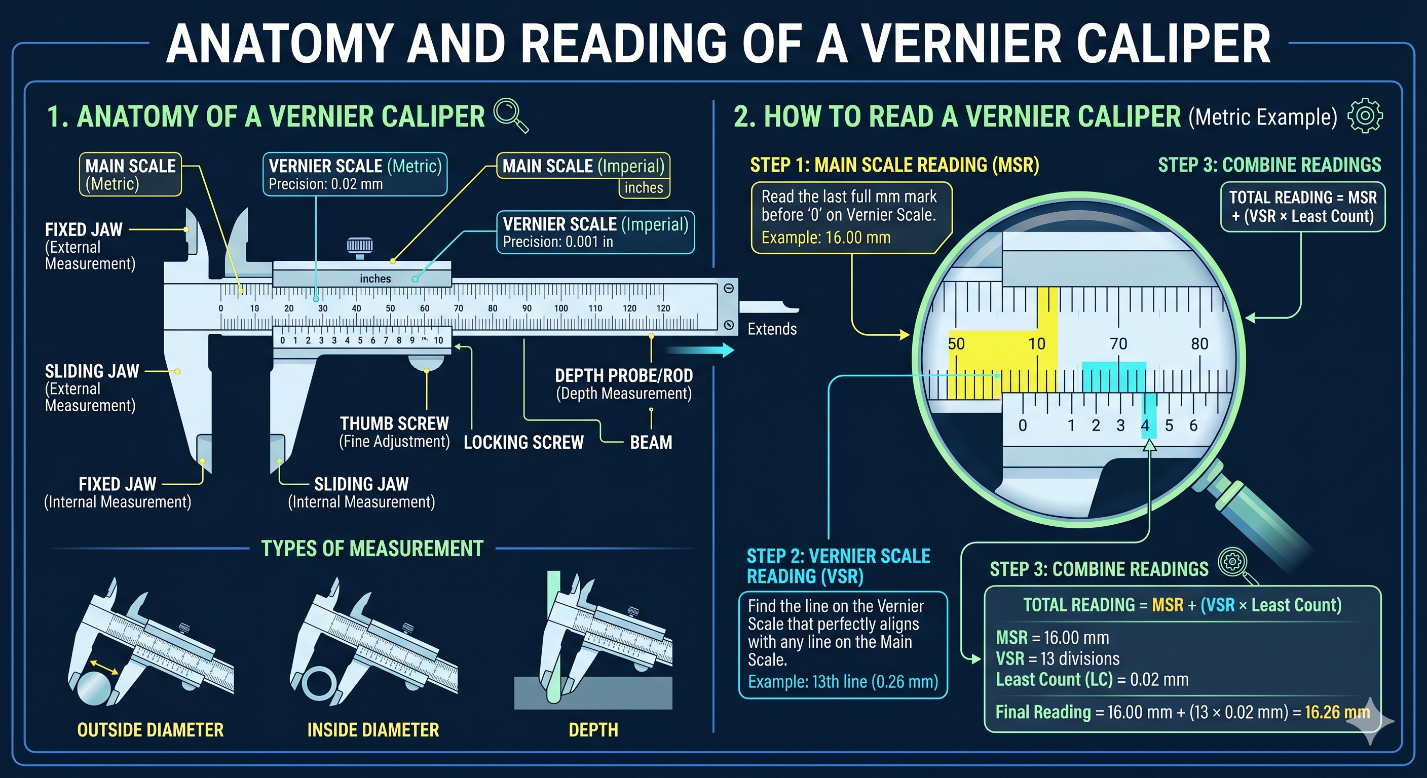
Anatomy and Reading of a Vernier Caliper

1. Finding the Least Count (LC):
The Least Count is the smallest value that can be measured accurately with the instrument. It is calculated as:

\text{Least Count (LC)} = 1\text{ Main Scale Division (MSD)} - 1\text{ Vernier Scale Division (VSD)}

Typically, $1\text{ MSD} = 1\text{ mm}$ , and $10\text{ divisions on the Vernier scale}$ align with $9\text{ divisions on the Main scale}$ ($9\text{ mm}$).
Therefore:

1\text{ VSD} = \frac{9}{10}\text{ MSD} = 0.9\text{ mm}

\text{LC} = 1\text{ mm} - 0.9\text{ mm} = 0.1\text{ mm} = 0.01\text{ cm}

2. Reading the Instrument:
To find the total reading:

\text{Total Reading} = \text{Main Scale Reading (MSR)} + (\text{Vernier Scale Coincidence (VSC)} \times \text{LC})

3. Accounting for Zero Error:
Sometimes, when the jaws of the caliper are closed, the zero mark of the Vernier scale does not align with the zero of the main scale.

Positive Zero Error: The Vernier zero lies to the right of the main scale zero. (Subtract this error from the final reading).
Negative Zero Error: The Vernier zero lies to the left of the main scale zero. (Add the magnitude of this error to the final reading).

Significant Figures in Calculations

Addition and Subtraction: Round the result to match the least number of decimal places of any number in the input.
$12.11\text{ (two decimals)} + 8.1\text{ (one decimal)} = 20.21 \rightarrow \text{rounded to } 20.2$
Multiplication and Division: Round the result to match the least number of significant figures of any input.
$4.56\text{ (three sig-figs)} \times 1.4\text{ (two sig-figs)} = 6.384 \rightarrow \text{rounded to } 6.4$

Advanced

Every experimental measurement is represented as $x \pm \Delta x$ , where $x$ is the measured value and $\Delta x$ is the uncertainty or error.

Classification of Errors

Systematic Errors: Constant errors that skew measurements in one direction (e.g., poorly calibrated instruments or zero errors). These can be eliminated by correction.
Random Errors: Fluctuations that occur unpredictably. These can be minimized by taking multiple readings and calculating the mean value.

If we take $n$ measurements of a quantity, the mean value $\bar{x}$ is:

\bar{x} = \frac{1}{n}\sum_{i=1}^{n} x_i

The Absolute Error for each measurement is $\Delta x_i = |x_i - \bar{x}|$ . The mean absolute error is:

\Delta x_{\text{mean}} = \frac{1}{n}\sum_{i=1}^{n} \Delta x_i

The relative error is $\frac{\Delta x_{\text{mean}}}{\bar{x}}$ , and the percentage error is $\frac{\Delta x_{\text{mean}}}{\bar{x}} \times 100\%$ .

Propagation of Errors

When calculating a final result from multiple measured quantities, errors propagate through the mathematical operations.

If two independent variables $A \pm \Delta A$ and $B \pm \Delta B$ are used to calculate a value $Z$ :

Mathematical Operation	Function	Maximum Absolute Error ($\Delta Z$)
Sum	$Z = A + B$	$\Delta Z = \Delta A + \Delta B$
Difference	$Z = A - B$	$\Delta Z = \Delta A + \Delta B$

For multiplication, division, or powers, relative errors must be added. If $Z = A^a B^b C^{-c}$ :

\frac{\Delta Z}{Z} = a\frac{\Delta A}{A} + b\frac{\Delta B}{B} + c\frac{\Delta C}{C}

Statistical Error Propagation (Quadrature)

If the errors in $A$ and $B$ are independent and random, simple addition of absolute errors overestimates the true uncertainty. Instead, we propagate errors in quadrature using partial derivatives:

If $Z = f(A, B)$ , then the standard deviation (uncertainty) $\sigma_Z$ is given by:

\sigma_Z = \sqrt{\left(\frac{\partial f}{\partial A}\sigma_A\right)^2 + \left(\frac{\partial f}{\partial B}\sigma_B\right)^2}

This relation ensures that independent uncertainties are combined geometrically, providing a more statistically robust estimate of experimental precision.